Unwarping diffraction patterns

Warped diffraction patterns are a common problem on SEM using a Snorkel lens to achieve high magnification. The magnetic field of the lens deviates the backscattered electrons which results in “warped” diffraction patterns. In most cases, the diffraction patterns (EBSPs) are non-indexable or the solution found is incorrect. To remedy to this problem, EBSD manufacturers offer in their acquisition software tools to unwarp the diffraction patterns as they are acquired. However, for some microscope, notably the Hitachi S4700 and SU8000 [1], and acquisition software, HKL Channel 5 SP9 [2], the proposed correction cannot compensate for the magnetic field.

Fortunately, on such system, the EBSPs can be stored on the local hard drive, unwarp using a third-party software and re-index in the EBSD software. This procedure is tedious and not so straightforward. The following paragraphs aim at giving a detailed tutorial of this procedure. Please contact me (pinard AT gfe DOT rwth-aachen DOT de) if some steps are unclear or if you find a mistake.

Summary

The unwarping procedure consists in 5 steps.

1. acquisition of diffraction patterns
2. acquisition of warped and unwarped diffraction patterns from a mono-crystal
3. making the shift maps between the warped and unwarped diffraction patterns
4. applying the shift maps to all the acquired diffraction patterns
5. re-indexing the diffraction patterns

Warning

The unwarping does not work in all cases. We found that this procedure does not work for correcting diffraction patterns from a BCC crystal structure (e.g. a-Fe). [3]

Requirements

The following software are required:

• LisPix (Note that some versions are more stable than others)
• EBSD-Image (optional, but recommended for speed gain)
• Flamenco (HKL Channel 5)

Acquisition

You should first acquire an EBSD map as you would do for any other mapping, except that you need to activate the option of saving all diffraction patterns. In Flamenco (HKL Channel 5), you need to go in the Image Storage tab of the workspace. If this tab is not visible, search Image Storage Page in the HKL Channel 5 manual to know how to activate it.

In the Image Storage tab, select the option from the combo box to Save a percentage of the patterns and enter 100%. You should also verify that the diffraction patterns are saved without any compression. We don’t want to loose any information from our EBSPs since we are going to re-index them.

Note

The preferences of the Image Storage tab may not always be saved in the user’s profile. You therefore have to always double-check that the option to save all diffraction patterns is activated before starting an acquisition.

For this acquisition, the use of the proper calibration and doing refining are not required as all the EBSPs are going to be re-indexed. It is however advisable to select the proper calibration to get an idea of the indexing rate of the mapping.

Technically, the procedure should work for any binning. It is however more difficult to establish the correction for highly compressed diffraction patterns. We would recommend using 4x4 binning, although we also successfully used 8x8 binning on some samples. [4] The 8x8 superfast binning should be avoided.

Finally, an important information that should be taken down is the working distance. Unless you are correcting the warping right after the acquisition, you will need the working distance of your mapping to acquire, in the next step, warped and unwarped diffraction patterns from a mono-crystal. Note that this information is not stored in the configuration file (CPR) of Flamenco.

Monocrystal

Once the acquisition is completed, the next step is to acquire two high quality diffraction patterns from a mono-crystal:

• one with the magnetic field (Snorkel lens) turned off (refer to as unwarped)
• another with the magnetic field turned on (refer to as warped)

For the type of mono-crystal, a silicon wafer gave us good results. These two diffraction patterns will allow us to find the correction, in other words, two shift maps. More on this in the next section.

It is important to acquire these EBSPs at the same working conditions as the EBSD mapping. The working conditions include:

• working distance
• beam energy
• beam current
• binning
• camera insertion position

Note

It is very important that the working distance is the same for the warped and unwarped diffraction pattern. Don’t forget to clear the hysteresis in the condenser lenses to get an accurate reading of the working distance.

For Hitachi microscope, since the working distance is not updated in the Low Mag (LM) mode, it is important to make an accurate alignment of the LM position in the Alignment menu.

The binning is also important as it has to match the binning used in the mapping. The shift maps obtained from the correction are dependent on the size of the diffraction pattern images (i.e. the binning).

Ideally, the acquisition of the warp and unwarp EBSPs would be performed immediately after the one of the mapping. However, this is often not possible unless one have a pre-tilted multi-samples holder and it is very time consuming as the correction must be repeated over and over again. We found that building a database of corrections to be a practical solution, in a similar fashion as the calibration of the EBSD detector is not repeated for every EBSD mapping, but selected based on the working distance and detector insertion position. Therefore, different corrections can be stored and used based on the working conditions mentioned above.

To acquire the warped and unwarped EBSPs, a high number of average frames should be selected to obtain high quality patterns. To know how to save a single diffraction pattern, please refer to the Saving EBSPs section of the HKL manual. Remember that you need to snap the diffraction pattern before saving it.

It is a good practice to save the two diffraction patterns in a directory named after the microscope conditions (e.g. 15kV_18mm_85mm_4x4). Note that we omitted the beam current as we assume that it was adjusted to properly saturate the camera. In this directory, two sub-directories should be created as they will be important for the next step: raw and corrected. The two diffraction patterns should be saved in the raw directory. This shift maps will be created in the corrected directory.

Shift maps

The shift maps are made using the freeware LisPix. More information about this image processing software can be found on its website which also gives a tutorial about unwarping images. This guide was inspired by this tutorial but is perhaps more adapted to the unwarping of EBSPs.

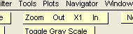
LisPix requires no installation; you only need to unzip the program. The interface of the software is slightly unconventional. Here is a quick overview. All the routines are accessed through the main menu bar.

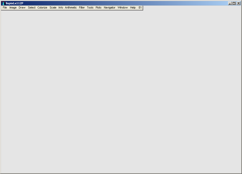
However, the menu bar can be expanded to access other important parameters. By repetitively clicking on the E1 button at the extremity of the menu bar until the label of this button becomes S, the zoom options and default read and write directories can be changed.

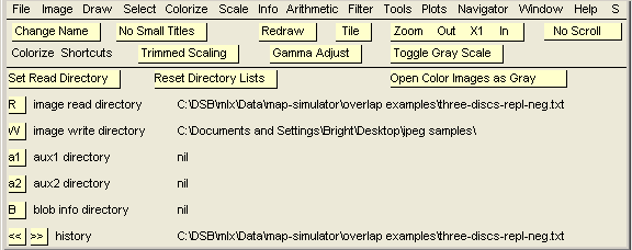
In the newly expanded menu, click on Set Read Directory and browse to the raw directory and select one of the two diffraction patterns. The selected directory should appear on the right of the image read directory label. Then, click on W and select Set from ^Read option. In the directory browser dialog, select the corrected directory. The full path of this directory should appear on the right of the image write directory label.

With our read and write directories setup, we can start the unwarping. This feature is under the menu Tools and Data Cube. The following window should appear.

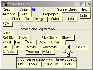
Change the write format to jpeg by clicking on Write button in the Data Cube window and selecting the option Set write type. Then click on Read button in the Data Cube window and select the option As Image Files. In the pop-up window, select both the warped and unwarped diffraction patterns by holding down the Shift key. An input box will then appear asking for a name of the cube. Enter any name or leave the default. A window with one of the image should appear as well as a slider at the bottom.

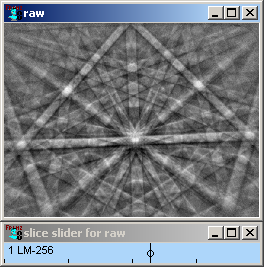
By moving the slider, you can see the two diffraction patterns. The next step is to click on Cube button in the Data Cube window to associate our newly created cube to the Data Cube tool. The name of the cube should appear next to the Cube button. We then need to tell the Data Cube tool which image is warped and unwarped. This is done by first selecting, using the slider, one image and then clicking on Ref Slc or Flick Slc button in the Data Cube window. Ref Slc should be the unwarped image and Flick Slc the warped one.

We can now start linking pixels in unwarped diffraction pattern to those in the warped one in order to establish the shift maps. This procedure is called Collect Tie Points. The goal is to find as many as possible shift vectors between the unwarped image and the warped one. LisPix will interpolate between these shift vectors to create the shift maps.

Before starting the collection of tie points, you can zoom in on the diffraction patterns to better see the pixels. Click on the button In in the expanded menu bar.

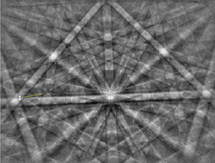
To start collecting tie points, click on the Warp button in the Data Cube window and select the option Collect Tie Points - ON. By hitting the Shift key you can toggle between the unwarped and warped diffraction pattern. Once you identified a feature in the unwarped diffraction pattern and found the corresponding one in the warped diffraction pattern, click on the pixel in the unwarped diffraction pattern, press and hold Shift and click on the pixel in the warped diffraction pattern. A yellow line (the shift vector) will appear on the diffraction pattern.

A few important points about collecting tie points:

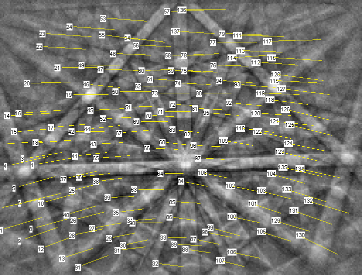
• You need about 80 to 100 tie points to obtain good shift maps
• The tie points should cover the whole diffraction patterns. It might be difficult to find matching pixels near the edges of the diffraction pattern as there is less signal there. Try your best.
• If you make a mistake, you can delete the last tie point collected by going in the Warp menu and selecting the option Delete Last Tie Point.
• It is better to use intersections of Kikuchi bands as matching features instead of intense pixels. Intersections can be more precisely identified.

Here is a typical result you would obtain:

Once you are done collecting tie points, press the Ctrl key. A text box will appear with the coordinates of the tie points. You need to save these information. Click on File and select Save Text. Save the tie points file in the corrected folder.

The next step is to create the shift maps. From the Warp menu, select Make warp shift maps. Two images appear: the x and y shift maps. You need to save these two images as RAW images. From the File menu, select Select Images & Cubes & Save as RAW. Using the Shift key, select the two shift maps and click OK. The shift maps are saved in the write directory, i.e. corrected folder.

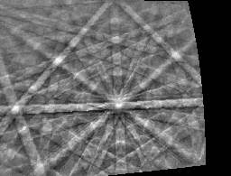
To see how these shift maps correct the warped diffraction pattern, open the warped EBSP by selecting the option Open from the File menu. Click on the image to select it and from the Warp menu, select Unwarp image. A dialog will pop-up asking you to select the x shift map and then another one to select the y shift map. The resultant diffraction pattern will appear in a new window. You need to save this diffraction pattern (File -> Save Image as JPEG) since it will be used to establish a new calibration.

Unwarping

Unwarping of the diffraction patterns stored during the mapping is performed with EBSD-Image. But before unwarping EBSPs, we need to re-organize some files and folders. Basically, we need to trick HKL Flamenco by creating a copy of our acquired mapping but replacing the diffraction patterns by the corrected ones.

Using Windows Explorer, browse to the location where you save your Channel 5 project. For a project called Project1, you should have:

• a CPR file: Project1.cpr
• a CRC file: Project1.crc
• JPG files if you check the function to acquire a SE or FSE image: Project1Before.jpg, Project1After.jpg, Project1BeforeWithOverlay.jpg
• a folder for the stored diffraction patterns: Project1Images

Take down the name of the latter folder, we will need it later. Create a folder CorrectedProjects and copy and paste the CPR, CRC and JPG files inside. Inside the CorrectedProjects folder, create a new folder with the exact same name as the folder containing the original stored diffraction patterns (e.g. Project1Images). We will tell EBSD-Image to save the unwarp diffraction patterns in this folder.

Open EBSD-Image and from the menu PlugIns, select EBSD -> UnWarp. A dialog will appear:

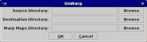
The source directory is the folder of the original diffraction patterns stored during the mapping. The destination directory is the newly created folder in the CorrectedProjects directory. The warp maps directory is the folder containing the two shift maps.

Warning

Be careful to never browse the folder containing the stored diffraction patterns. Windows does not handle folders with many files in them. It may take up to a minute for Windows to display the files in it.

EBSD-Image will perform the correction on the first EBSPs and show you the result before continuing with the other diffraction patterns. Verify that the correction is done properly and click OK. The progress bar at the bottom-left corner indicates the completion percentage.

Re-indexing

The re-indexing procedure is exactly the same as any re-indexing done in HKL Flamenco. We therefore refer the readers to the Re-analysing Projects Offline section of the HKL manual for more information.

The first step is to create a new calibration using the corrected EBSP. A new calibration needs to be established as the correction of the warped EBSPs has most likely shift the position of the pattern center. From the menu EBSP, select Open and open the corrected EBSP (i.e. the warped diffraction pattern used to create the shift maps that was then corrected with the shift maps). Select the phase of the mono-crystal. Go in the EBSP Geometry tab of the workspace and adjust the region of interest (green circle). The region of interest should not include any black region around the corrected diffraction pattern. In the Band detection tab, select the Band Edges detection and increase the maximum number of detected bands to 8. Index the diffraction pattern and improve the calibration using the Refine function. Save this calibration in the corrected folder (where the shift maps are saved). You could re-used this calibration to re-analyze mappings acquired at the same working conditions.

Warning

The calibration should always be set prior to starting the setup of a re-analyzed project.

From the Projects menu, select Open and then Reanalyze project. A dialog will appear asking you to select a project to re-analyze. Browse to the CorrectedProjects directory and select the project CPR file. The following dialog will then appear:

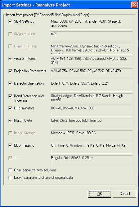
Uncheck the following options:

• Area of interest
• Projection parameters

We are not importing these information from the original project as we want the re-analyzed project to use our new calibration and region of interest.

The following dialogs may appear:

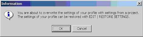
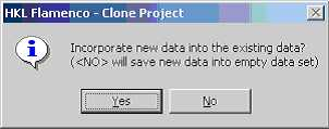
Click OK or YES.

A new job is created. Add this job to the Job list and click Run. You may want to pause the re-analysis and fine tune the calibration. You can always run again the re-analysis.

That’s it!

---

[1]	Hitachi S4700 and SU8000 are a registered trademark of Hitachi High-Technologies Inc.

[2]	HKL Channel 5 is a registered trademark of Oxford Instruments plc.

[3]

From a personal conversation with a former lead engineer of HKL, higher constraints hard coded in HKL Flamenco seem to be the reason explaining this problem. Even after the warping correction, the Kikuchi bands are not as “straight” as regular Kikuchi bands coming from diffraction patterns not affected by the magnetic field.

[4]	Binning dimensions correspond to the Nordlys II camera.