What is an experiment?

In EBSD-Image, the procedure of going from diffraction patterns to indexed solutions is called an experiment. This includes, of course, several steps such as the Hough transform, peak detection and various other computations. It is the core of the EBSD-Image module. All the features, options and file formats in this module are used at one point or another by the experiment engine.

The following paragraphs explains the structure and the fundamental concepts of the engine. For a walkthrough guide on setting up an experiment and running it, please refer to How to run an experiment guide.

Objectives

The design objectives of the experiment engine can be summarized by one word: flexibility. As a research and development tool, one should be able to adapt the experiment to match their specific needs. No hidden information or fudge factor. One should also be able to specify the outputs they want as well as all the steps to obtain these results. In summary, the users are given three levels of flexibility:

• To decide the steps towards an output
• To change any parameters
• To implement new algorithms inside the engine

Structure

The engine can be simplified into three parts:

1. Inputs
2. Operations
3. Outputs

Inputs

As mentioned before, the inputs of the experiment are diffraction patterns. An experiment can be the analysis of one or a million diffraction patterns depending on the user’s needs, however each diffraction pattern is independently processed.

Patterns can be loaded from an image file, a folder containing many image files or an SMP file. The latter is a format specific to EBSD-Image. It allows to store a large quantity of diffraction pattern images in our file and load these images quickly.

Operations

We refer to the steps in the experiment as operation. They are closely related to the various type of maps available in RML-Image and EBSD-Image. An operation is a process taking one or many inputs and returning one or many outputs. The input(s) and output(s) are known a priori.

Major steps

An experiment can be divided into five major steps:

1. Pattern operations

   The pattern operations consist in loading the diffraction pattern image and performing image analysis routines to enhance the pattern, remove noise, select a region of interest, etc.

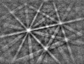
Initial diffraction pattern.

2. Hough operations

   The Hough operations are related to the Hough transform. This algorithm is used to transform the image space into the Hough space. The Kikuchi bands in the diffraction pattern are converted to peaks. One can select the resolution of the Hough transform, operations to select a region of the Hough space, etc.

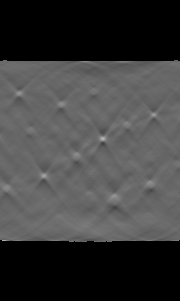
Hough map.

3. Peak detection operations

   The next step is to located the peaks in the Hough transform. First algorithms such as the butterfly convolution mask can be used to selectively enhance the peaks in Hough space. Different peak detection algorithms are available to perform a thresholding of the Hough map.

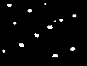
Location of the detected Hough peaks.

4. Peak positioning operations

   The result of the previous step is a binary map. Therefore, the next step is to identify the peaks by measuring their position in the Hough space (\(\rho\) and \(\theta\)) as well as their intensity. Operations to clean unwanted peaks or to look for specific peaks can be performed as part of this step.

5. Indexing operations

   Finally, using the identified Hough peaks, the indexing can be performed. In other words, the orientation and the phase of the initial diffraction pattern is calculated. A goodness of fit value is also provided to evaluate how closely the solution(s) match(es) the identified Hough peaks.

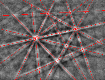
Overlay of the solution on the initial pattern.

Categories

More specifically, the five major steps can be subdivided into sub-steps or categories. Overall, the experiment engine goes through 18 categories of operations. Some categories can contain more than one operation, some can contain no operation and other can only contain one. The categories follow a logical chain of actions: the input of operation 2 is the output of operation 1 and the output of operation 2 will be the input of operation 3.

Each major step, previously discussed, contains 4 categories of operations except for the first one which only has 2 (4 x 4 + 2). Each group follows the same logic:

• An single operation which defines the group
• A set of operations to process the input(s) of this single operation
• A set of operations to process the output(s) of this single operation
• Finally, a set of operations to compute result(s) from this single operation

In order this gives:

• Pre-operations
• Operation
• Post-operations
• Results operations

Note

The pre, post and results operations can contain zero or many operations, whereas the category operation can only contain one operation.

In summary, the experiment engine will process each category of operations as follows:

1. Pattern post-operations
2. Pattern results operations
3. Hough pre-operations
4. Hough operation
5. Hough post-operations
6. Hough results operations
7. Peak detection pre-operations
8. …

A description and an example of a potential operation is given for each category in the following table:

#	Group	Category	Description	Example
1	Pattern	Post	Process the diffraction pattern after it being loaded	Selecting the region of interest
2	Pattern	Results	Compute results from the diffraction pattern	Quality index using the pixels average
3	Hough	Pre	Process the diffraction pattern before the Hough transform	Median
4	Hough	Operation	Perform the Hough transform	Hough transform with a resolution of 0.5 deg.
5	Hough	Post	Process the Hough transform	Truncate edges
6	Hough	Results	Compute results from the Hough transform	Quality index from the range of the Hough
7	Peak detection	Pre	Process the Hough transform prior to the peak detection	Butterfly convolution
8	Peak detection	Operation	Detect the peaks in the Hough transform	Top hat thresholding
9	Peak detection	Post	Process the detected peaks to remove unwanted peaks	Remove small peaks
10	Peak detection	Results	Compute results from the detected peaks	Quality index using the number of detected peaks
11	Peak positioning	Pre	Process detected peaks prior to their positioning	Keep only peaks of a certain shape
12	Peak positioning	Operation	Identify Hough peaks (position and intensity) from the detected peaks	Find the position using the local centroid of each peak
13	Peak positioning	Post	Process the identified Hough peaks
14	Peak positioning	Results	Compute results from the identified Hough peaks	Image quality index
15	Indexing	Pre	Process the Hough peaks before the indexing	Select most intense peaks
16	Indexing	Operation	Index the Hough peaks to potential solutions (phase and orientation)	Automated indexing from Krieger Lassen
17	Indexing	Post	Process the solutions to find the best one	Lowest misfit
18	Indexing	Results	Save orientation and phase of the solution	Euler angles

Input(s) / Output(s)

Each category is defined by a distinct set of inputs and outputs. A summary of each category is given in the following table.

#	Group	Category	Input(s)	Output(s)
1	Pattern	Post	ByteMap	ByteMap
2	Pattern	Results	ByteMap	array of byte or float
3	Hough	Pre	ByteMap	ByteMap
4	Hough	Operation	ByteMap	HoughMap
5	Hough	Post	HoughMap	HoughMap
6	Hough	Results	HoughMap	array of byte or float
7	Peak detection	Pre	HoughMap	HoughMap
8	Peak detection	Operation	HoughMap	BinMap
9	Peak detection	Post	BinMap	BinMap
10	Peak detection	Results	BinMap	array of byte or float
11	Peak positioning	Pre	BinMap	BinMap
12	Peak positioning	Operation	BinMap and HoughMap	array of Hough peak
13	Peak positioning	Post	array of Hough peak	array of Hough peak
14	Peak positioning	Results	array of Hough peak	array of byte or float
15	Indexing	Pre	array of Hough peak	array of Hough peak
16	Indexing	Operation	array of Hough peak	array of Solution
17	Indexing	Post	array of Solution	array of Solution
18	Indexing	Results	array of Solution	array of byte or float

Outputs

All the outputs of the experiment engine are saved in an EbsdMMap. In short, a multimap is a container of many maps, all sharing the same image dimensions. A new map is created for each result. For example, the image quality is saved in a RealMap and the orientation (given as a quaternion is saved as four RealMap, one for each coefficient of the quaternion. There is no limit or restriction on what type of results can be saved, as long as a result can be expressed as a number or a set of numbers.

The dimensions (width and height) of the result maps inside the EbsdMMap depends on the size of the mapping. If only one diffraction pattern is analyzed, the maps have a 1x1 dimension.

The operations used in the experiment and their parameters are saved in a human readable and editable XML file located in the working directory.

Analysis

All the results maps can be viewed and used to extract more information in EBSD-Image. For more information on this, refer to Analyzing results.